Custom Data

Use source = "custom" when project-owned data should be authoritative. This is common for production studies, teaching material, offline CI, and cases where public providers are incomplete or too volatile.

Path resolution

Relative path and mask_path values are resolved from the TOML file. For typed data sections, bare filenames can also be resolved against the workspace data/ folder and the matching data/<family>/ folder.

[data]
project_crs = "EPSG:2154"
types = ["dem", "geology", "hydrometry", "recharge"]

[[data.dem.sources]]
source = "custom"
path = "data/dem/catchment_dem.tif"

Local rasters and grids

Custom gridded climate and hydrological inputs can be read from NetCDF or GeoTIFF files. NetCDF time dimensions are sliced to the project period when a period is available.

[data.recharge]
date_start = "2000-01-01"
date_end = "2002-12-31"

[[data.recharge.sources]]
source = "custom"
path = "data/recharge/recharge_daily.nc"
source_unit = "mm/day"

Set source_unit when the file metadata is absent, ambiguous, or not the unit expected by HydroModPy. This is safer than compensating later in solver parameters.

DEM custom inputs use the DEM loader and can read common raster formats used by the DEM manager:

[[data.dem.sources]]
source = "custom"
path = "data/dem/local_dem.tif"
mask_path = "data/masks/watershed.gpkg"

The expected output is the same kind of basin-support panel as for public providers: a readable DEM, a coherent watershed boundary, and no CRS surprise.

A custom DEM should make this support check boring. If the basin appears shifted, cropped, inverted, or empty, fix the local file metadata before changing solver settings.

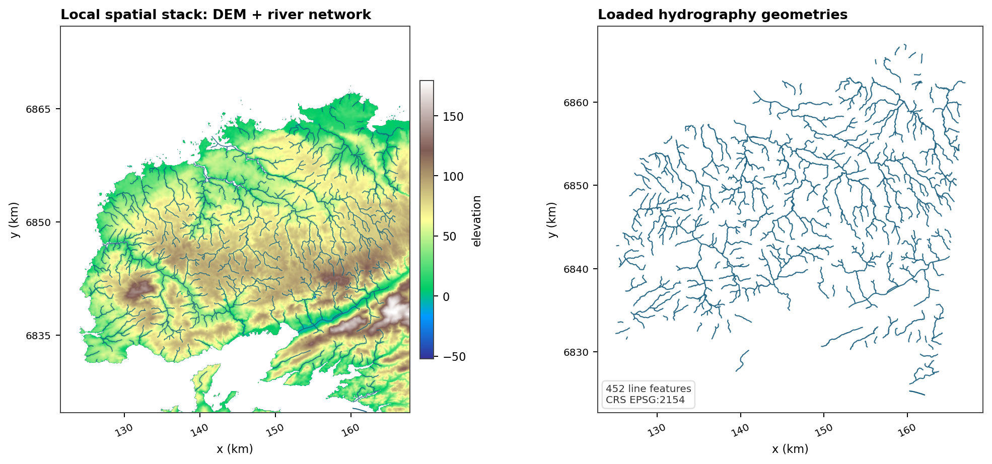
Fig. 130 The generated local example shows the same custom-data principle on a smaller support: the raster and vector layers must agree spatially before any downstream workflow trusts them.

Local vectors

Custom geology vectors need a field that carries the geology code:

[[data.geology.sources]]
source = "custom"
path = "data/geology/geology.gpkg"
code_field = "CODE_LEG"
values_table_path = "data/geology/hydraulic_properties.csv"

The rendered geology panel should expose both the spatial units and their legend. The important check is that the geology code used by code_field is still interpretable after loading, clipping, reprojection, and optional joining with the hydraulic-property table.

A custom geology layer is ready to drive supports, zones, or hydraulic parameters only when the displayed polygons and legend are readable together. Missing labels, collapsed categories, or unexpected empty zones usually point to a ``code_field`` mismatch, a failed attribute join, or a CRS issue in the source vector.

Custom hydrography can point to a local river-network vector:

[[data.hydrography.sources]]
source = "custom"
path = "data/hydrography/rivers.gpkg"
rasterize_field = "FID"

For local hydrography, the visual contract is the same as for BD Topage or OSM: the loaded river layer must make sense on the basin support.

Custom river data is authoritative only after it has passed this spatial check. A correct file path is not enough.

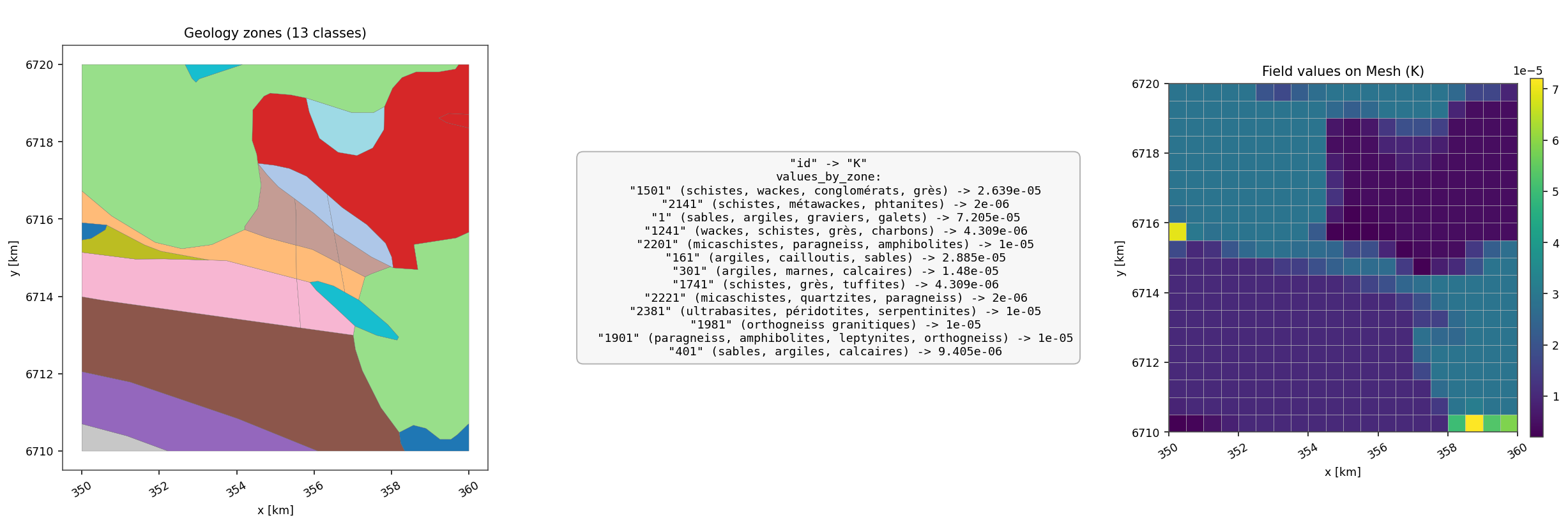
Fig. 133 Local vector data can also become model-facing parameters. Here the geology code joins to a K table, then the result is transferred to a mesh field.

Local point and time-series folders

Point/time-series custom sources use a directory convention:

data/hydrometry/
|-- hydrometry_custom_LOC.csv
|-- hydrometry_custom_J1234010_20000101_20021231_D.csv
`-- hydrometry_custom_J1234020_20000101_20021231_D.csv

The location file defaults are:

Column	Meaning
id	Station identifier used to find chronicle files.
x, y	Station coordinates.
crs	Optional CRS per station. default_crs is used when the column is missing.
unit	Source unit for point records when the family requires unit conversion.

Chronicle CSV defaults are datetime and value. Rename columns in TOML instead of reshaping source files:

[data.hydrometry]
date_start = "2000-01-01"
date_end = "2002-12-31"

[[data.hydrometry.sources]]
source = "custom"
path = "data/hydrometry"
col_id = "station"
col_x = "lon"
col_y = "lat"
default_crs = "EPSG:4326"
col_datetime = "date"
col_value = "Q"
station_ids = ["J1234010"]

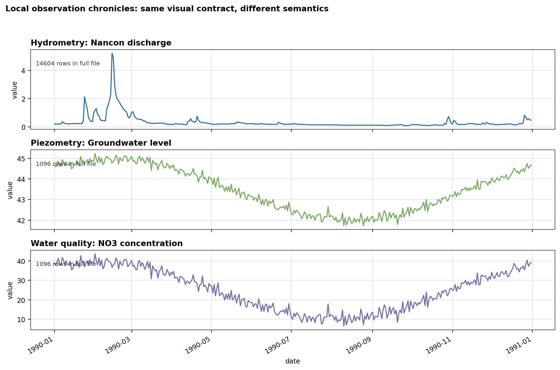
Fig. 134 The same directory convention can carry discharge, groundwater level, or chemistry. The chronicle figure is where units, gaps, and temporal coverage become visible.

The overview panels should then show both the selected stations and the chronicles that were actually ingested.

For custom time series, the most useful check is not the filename convention itself but the rendered chronology: dates, gaps, units, and station identity must be visible before a solver or calibration run reuses the data.

Controlled sources

Some sources are local by design even when they do not read a file.

[data.oceanic]
date_start = "2020-01-01"
date_end = "2020-12-31"

[[data.oceanic.sources]]
source = "constant"
value = 0.0

[data.recharge]
date_start = "2020-01-01"
date_end = "2020-01-31"

[[data.recharge.sources]]
source = "synthetic"
values = [0.8, 1.2, 0.6]

Use constants and synthetic forcing for tests, tutorials, and controlled diagnostics. Use custom files when the goal is to reproduce a production data set.