
Simulated Active Network#
Purpose#
The simulated active network is the part of the drainage support that becomes active because of the groundwater-flow solution.
It is not loaded from an external river file and it is not the DEM-derived
generated hydrographic network. It is a post-processed signal derived from
cell-by-cell simulated drainage outflow.
This page explains the three levels that should not be confused:
local drain outflow at each cell,
downstream accumulation of that outflow,
a thresholded or persistence-based active-network mask.
Conceptual Contract#
HydroModPy keeps the raw simulated drainage signal as cell fields before any vector network is declared.
For a steady-network question, distinguish the steady-flow scenario from the
transient occupancy rule. A simulated steady active network should preferably
be derived from a representative flow_regime = "steady" run, then compared
with the observed reference network. The transient always_active mask
only means active at all timesteps of the analysed chronicle.
Field or view |
Meaning |
How to read it |
|---|---|---|
|
Positive groundwater discharge through drains, summed over model layers. |
Local source term. A positive value means that groundwater leaves the aquifer through the drain condition in that cell. |
|
Downstream accumulation of positive drain discharge. |
Network signal. High values mark cells that receive upstream active drainage contributions. |
|
Boolean or continuous mask derived from |
Display and metric layer. The threshold and time rule must be explicit. |
The sign convention is intentionally normalized at the HydroModPy result level:
outflow_drain is positive when water leaves the groundwater system. This is
different from raw MODFLOW cell-budget records, where leaving the aquifer is
usually stored with a negative sign.
Why Accumulation Is Not Just Another Drain Map#
outflow_drain and accumulation_flux answer different questions.
outflow_drain answers:
“Where does the model release water locally through the drainage package?”
accumulation_flux answers:
“If local drainage contributions are routed downslope through the mesh, which cells form the connected active drainage structure?”
This distinction matters because a downstream cell may have a small local drain outflow but a large accumulated flux if many upstream cells drain toward it. In figures, this usually makes confluences and persistent branches easier to see.
Where This Page Fits In The Examples#
Use this page as the MODFLOW 6 result-contract example. It shows how a solver run becomes an interpretable active-network diagnostic:
head -> outflow_drain -> accumulation_flux -> simulated_active_network
For the complete list of examples, commands, and files to open, see Worked Examples. For the current distinction between supported fields, demonstrated examples, and non-contracts, see Status And Limitations.
MODFLOW 6 Validation Example#
The following figures come from a real MODFLOW 6 run executed through the HydroModPy simulation workflow. The run has three stored timesteps and a structured 60 x 60 MODFLOW 6 support. The MODFLOW 6 extractor writes the solver mesh topology from the grid binary file, so the result layer can reshape fields on the solver grid instead of forcing the original DEM shape.
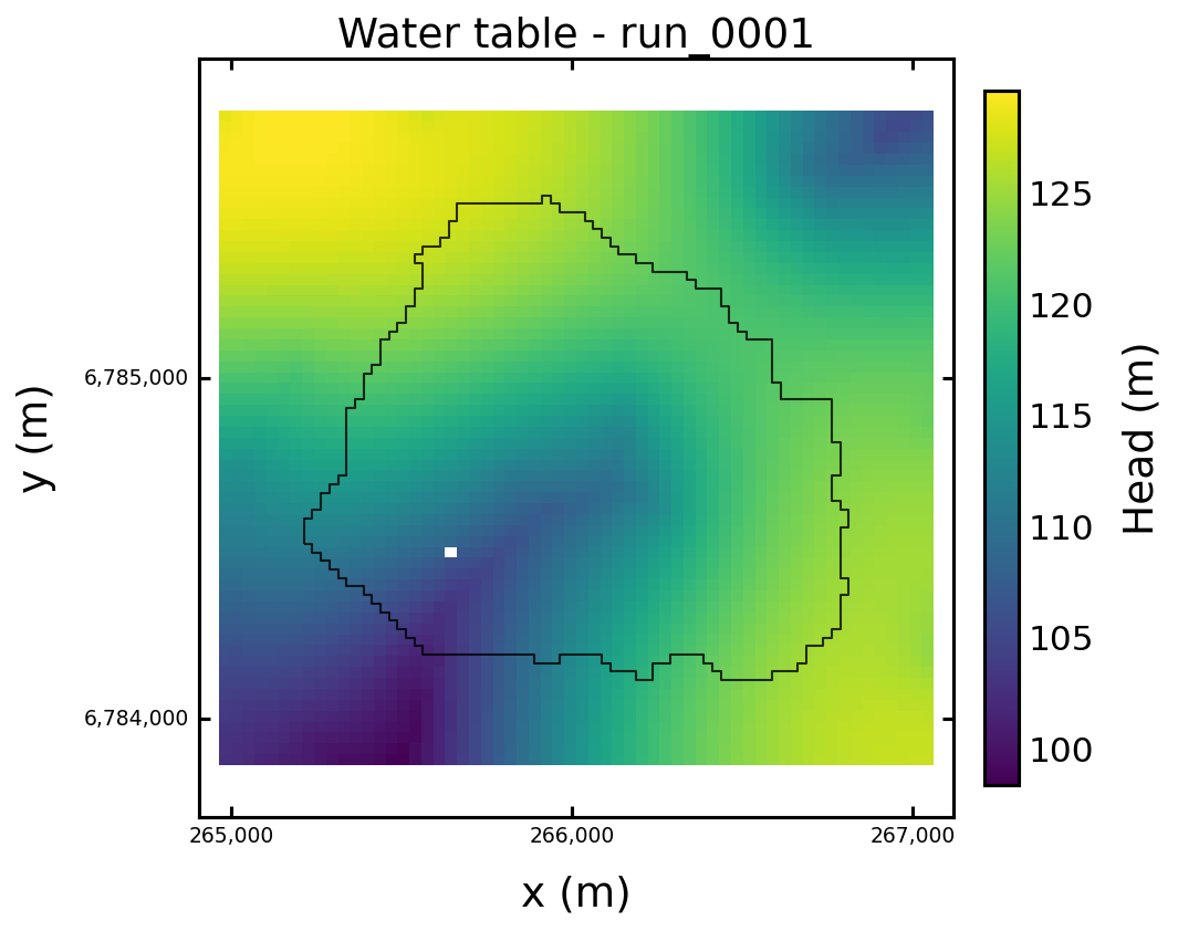
Fig. 28 Water-table field for the validation run. This is the groundwater state from which head-dependent drainage outflow is produced.#
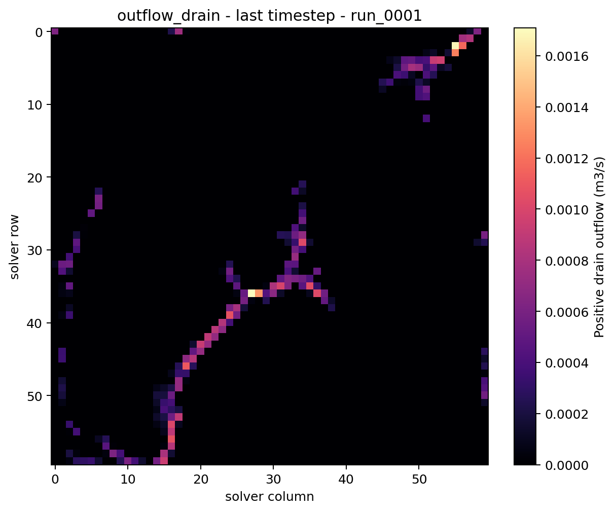
Fig. 29 outflow_drain on the last timestep. The field is local and positive:
it shows where groundwater leaves the aquifer through the drain condition.#
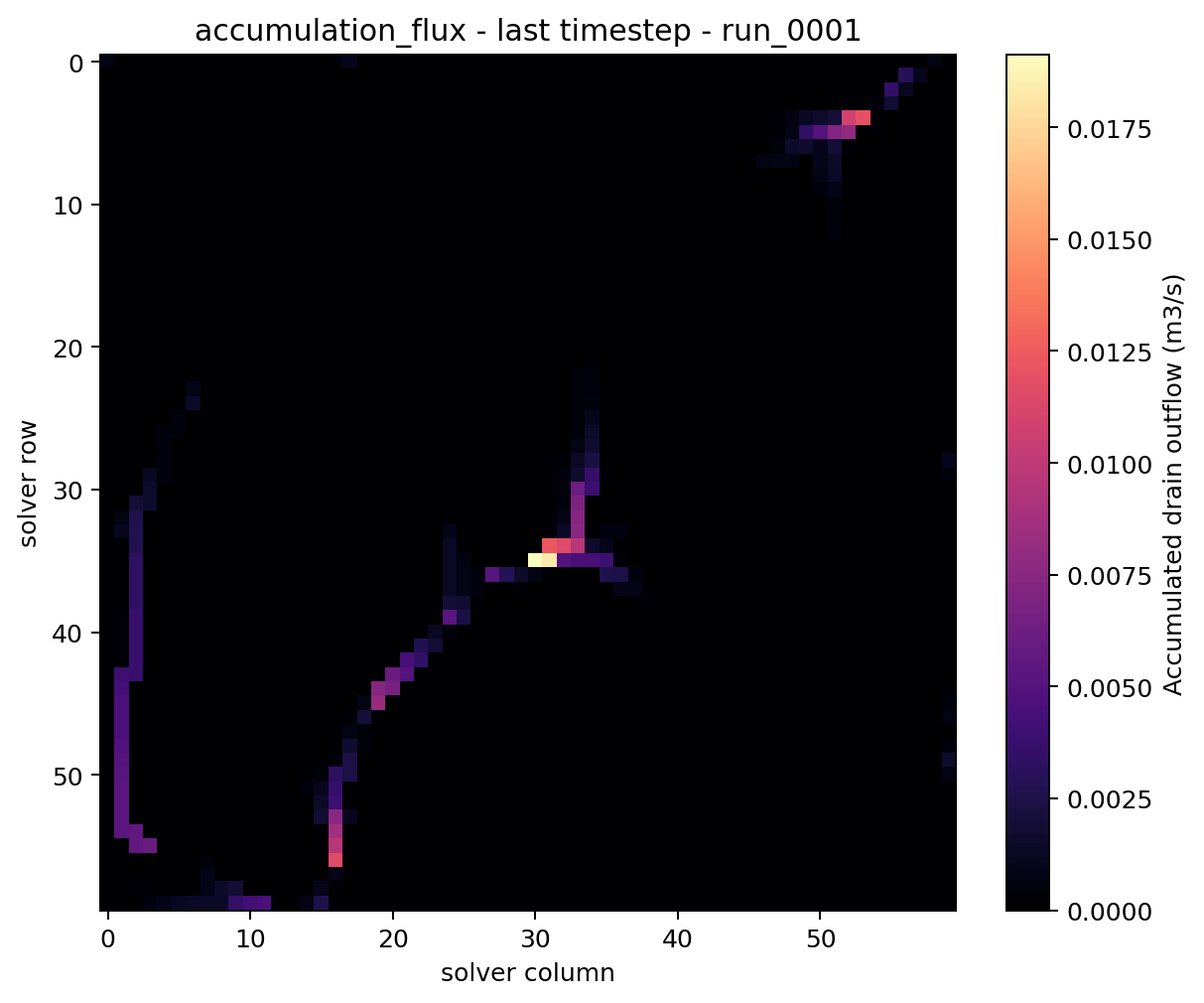
Fig. 30 accumulation_flux on the last timestep. The spatial pattern follows
the same active-drainage support, but values increase along downstream
paths because upstream contributions are accumulated.#
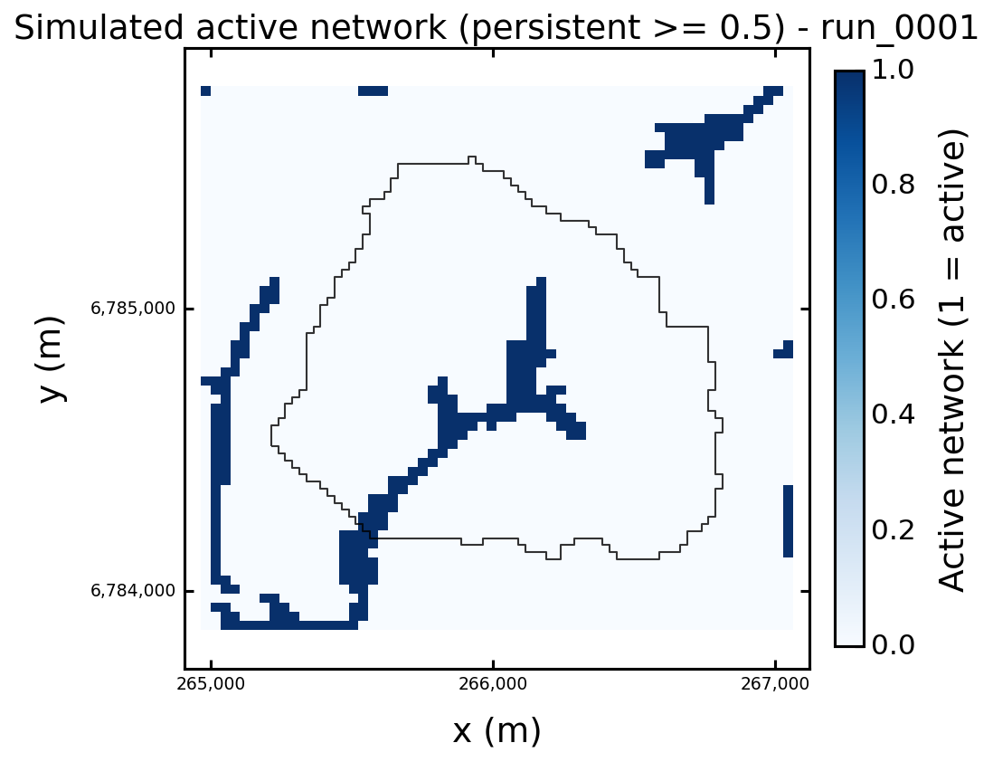
Fig. 31 simulated_active_network figure. This is a computed cell-mask view
produced from accumulation_flux. It is useful for inspection and
comparison, but it is not yet a stored vector line network.#
For this validation run, the last timestep diagnostic summary was:
Field |
Shape |
Max |
Sum |
Non-zero cells |
|---|---|---|---|---|
|
|
|
|
|
|
|
|
|
|
Do not interpret the sum of accumulation_flux as a water-budget total. It
is a routed network diagnostic: the same upstream water contribution may be
counted again along downstream cells. Use budget tables and outflow_drain
for mass-balance interpretation.
Current MODFLOW 6 Implementation Path#
For flow/modflow6, HydroModPy now uses the following result path:
MODFLOW 6 produces heads and budget components.
The output adapter reads the MODFLOW 6 grid binary file when available.
The catalog stores:
mesh/vertices,mesh/face_node_connectivity,mesh/topography,mesh/z_interfaces.
The derived-field extractor converts raw DRN budget values to positive
outflow_drain.The extractor computes
accumulation_flux:structured D8 routing when a regular raster support is available,
mesh-graph downhill routing when a plottable face connectivity exists,
local positive outflow as a conservative fallback.
Run.fields(...)returns fields on the solver support when that support differs from the geographic DEM grid.The display layer enables
simulated_active_networkwhen bothaccumulation_fluxand plottable mesh topology are present.
Programmatic Reading#
After a run is available through Run, inspect the fields directly:
Render the active-network figure when the capability is available:
if "simulated_active_network" in run.display_capabilities:
    run.plot("simulated_active_network", save="figures")
Compare the same active-network view against the observed reference
network when that role exists:
overlap = run.cell_field_network_overlap_metrics(
    network_role="reference",
    variable="accumulation_flux",
    mode="persistent",
    threshold=0.0,
    persistence_threshold=0.5,
)

distance = run.cell_field_network_distance_metrics(
    network_role="reference",
    variable="accumulation_flux",
    mode="persistent",
    threshold=0.0,
    persistence_threshold=0.5,
)
overlap gives coverage, precision, F1 and Jaccard on mesh cells.
distance gives bidirectional planar cell-centroid distances. It is a
current diagnostic, not the future downslope DEM-routing criterion.
For steady runs, do not pass a time mode unless you intentionally want to force a diagnostic snapshot. The default is the steady-state active-network field:
mask = run.cell_field_active_mask(
    variable="accumulation_flux",
    threshold=0.0,
)
For transient runs, select the time rule explicitly:
mask = run.cell_field_active_mask(
    variable="accumulation_flux",
    mode="persistent",
    threshold=0.0,
    persistence_threshold=0.5,
)
The main modes are:
last: active cells on one timestep;any: active at least once;persistent: active for at least a declared fraction of timesteps;always_active: active at every analysed timestep;persistence: continuous active-time fraction.
Use steady for the representative steady-flow concept. The transient
always_active mode only means active at every stored timestep of the chosen
analysis window, and should not be used as a synonym for a steady active
network.
What This Is Not Yet#
The simulated active network is currently a computed cell-mask and metric
layer. HydroModPy does not yet automatically persist a canonical vector feature
named hydrographic_network_simulated_active.
That distinction is deliberate.
Before vectorization becomes a stable contract, the project still needs to choose:
the default activation threshold;
whether the canonical representation is one steady network, one transient summary, or several named networks;
how much simplification or line extraction should be applied;
whether the first canonical representation should be raster-like, vector-like, or both.
Until those choices are fixed, the safest interpretation is:
use
outflow_drainfor local drainage outflow and budget reasoning;use
accumulation_fluxfor active-branch detection;use
simulated_active_networkfigures and overlap metrics for inspection;do not assume that a stored vector hydrographic-network role exists.